
4D tomography: walkthrough of my project - part 3
- Published
- in algorithms, experimental math, inverse problems, mathematics, medical imaging, physics, research, talks
Here comes the final part of the walkthrough of my current project on dynamic sparse tomography (see also part 1 and part 2). In the previous post I left the question of the choice of the cut-off function  hanging. In a classical level set method, would be the Heaviside step function. The Heaviside function is defined as:

When the first tests on the static case were ran, Kolehmainen, Lassas and Siltanen noticed that the reconstruction was not good, but the level set function itself resembled the infinite precision data. Hence, they decided to use a new cut-off function:

that is the identity function, with a non-negativity constraint. In my own simulations, I approximated the latter by a  map:
map:

Numerical results were slightly better and the corresponding objective functional was Frechet differentiable (not only Gateaux differentiable, as before).
Recently Niemi et al. proved that  is equivalent to the non-negativity constraint Tikhonov functional. Hence, they generalized it to higher orders. For instance, the functional of order 2 to minimize is:
In this case, existence of a global minimizer was proved.
The first simulation Esa Niemi ran, was on the (2+1)D phantom shown in part 2. The intensity value of the medium is constantly 1, while outside it we have a background constant at value 0. At each time frame, measurements were collected around a full-angle, from only 7 equally distant directions. In the following chosen time frames (“sections” of the 3D surface) you can see the outcome.

The first column depict the infinite precision data, that is the simulated body. In the second column the same sections are reconstructed through Filtered Back Projection, that is the method currently used by industrial machineries. FBP does not work with undersampled data, as you can see. In the third and fourth column you can compare the reconstructions by the level set method I explained, respectively by the order 1 and the order 2 functionals. In the last column, I show how a classical regularization method works in this case, namely Tikhonov regularization. Our new method, with the order 2 functional, works much better, as you can see by the approximation errors shown in each frame.
The second step Esa faced was testing on real data. To reproduce the same measurement setting of the simulation, he created a stop-motion animation. He put some sugar cubes and measured around a full-angle. Then he added one or a couple of sugar cubes and measured again, and so on. The new sugar cubes represented the dynamic change (sudden, in this case) in the data. Sugar cubes are also a good choice because they have corners, which the simulated data was missing. The results can be seen in the following pictures (I selected only three time frames).

The first column shows a fine reconstruction, done by FBP, using many projection angles. From the second column on, only 10 projections were used. Our method is compared with another classical reconstruction method, as Total Variation is. Again, the outcome is very promising: of course in this case you cannot compute an approximation error but you can compare visually with ground truth.
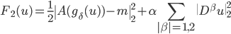
There is still an extensive investigation to carry on. Personally, one of my next goals is to make the codes work in a more realistic measurement setting, namely helicoidal acquisition. I would like to sample the data while the dynamic change happens. To this purpose, I designed the following prototype, inspired by the potential application of angiography.
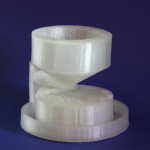

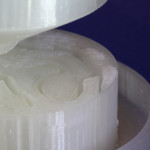
The top part of the model has the practical purpose of collecting the viscous contrast agent and buy some time for it while we start the measurement procedure. The relevant part of the model are the “veins” that would be (slowly) filled up while we rotate the sample and acquire the data. This will be the next (2+1)D real data I will test on. Currently I am experimenting to find the right contrast agent together with my colleague Alexander Meaney. In the meantime I am experimenting with simulated data with promising results.
This is the current state of my project. Personally, I find it to be a perfect mix of theoretical aspects, computer simulations and great potential for applications. I also hope this will make me get in touch with professionals of other areas. For instance, it would be nice to get suggestions for testing data, or measurement settings. So… feel free to comment and share your view.