A small guide to Random Forest - part 1

I've recently started playing with Kaggle and got curious about one of the most famous classification/regression framework, Random Forest. In a problem of classification or regression, several random decision trees (a "forest") are built and at the end the outputs are combined ("bagging"). The intuition is that randomness and a meaningful quantity of trees will avoid over- and underfitting. One possible bagging technique is the majority vote. Take the case of predicting a binary outcome, say a random variable Y which can assume only values in , with respect to some features (occurred events). We assume there exist a correct answer - the "right model" - which we have to predict. The intuition of the majority vote is that if such "divine truth" exists and we build several "quite reasonable" models, most of them will give the right prediction. If the right value is and we make "reasonable" predictions , most of them will be equal to 1 and only a minority will be equal to -1. In mathematical terms, we'll choose the following prediction:

(1)

Bagging is done in other ways, but to me the majority vote example is an easy way to understand the fundamental concept.
The Random Forest framework was introduced by statistician Leo Breiman in 2001 in his seminal paper. Even though implementations have been released in many languages (R, MatLab, Python, Java...), it's important to learn the basics, to be able to tune the parameters well.

Decision trees

The elements of a Random Forest are usually decision trees (there are variants of the framework, though). Assume we have the following database:
training data =
Each column is a sample, each row corresponds to a feature. We consider a binary output: . We now will choose random features (to be able to represent the problem in the plane) and will start building a decision tree. Assume our random sample is:
random sample =
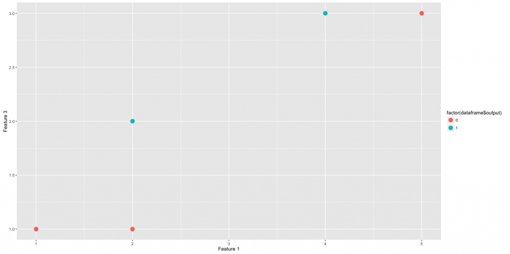
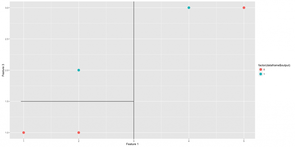
meaning that we randomly selected the features 1 and 3. Let's represent these points on a plane, assigning a different color on the base of the associate output.

Notice the distribution of points in this universal region:

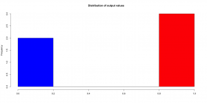
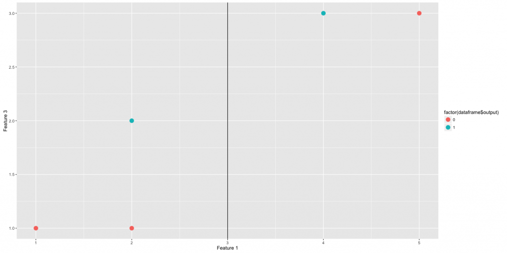
Now an hyperplane is selected (randomly or with some criteria, for instance maximising information gain) and the points are separated into two regions:

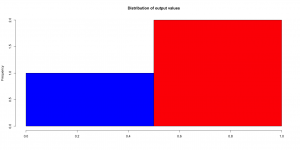
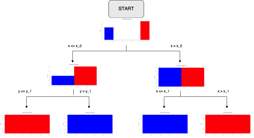
Our decision tree starts and we have the following split and new frequency distributions in the two new regions:

START

Now the idea is to iterate this procedure separately on each branch. For instance, we consider only Region 1 () and draw another hyperplane, say :

On the other branch, we draw another hyperplane :

Summing up, we built the following tree.

At this point clearly we can stop. We divided the plane in regions which completely classify our training data.
To summarise, here are the steps of Random Forest:

1. For k = 1, 2, ..., Ntrees:
   --> select a bootstrap sample S from training data
   --> grow a decision tree (with a stopping criterion for the depth)
2. Bagging on

Next, I plan to show the use of some variables and features of the randomForest R package and to make some observations on the algorithm. For instance, how to choose Ntrees? How to determine a reasonable stopping criterion for the tree depth?

The featured image is an excuse to introduce a great visualisation resource for Random Forests: check it out.

Facebook

Linkedin

Twitter

email

Print